This page describes the construction and operation of a device for testing rocket motors. It allows the recording of the thrust generated by the motor during a static test. The recorded data is then analysed using an Excel spreadsheet.

This load cell amplifier is a little different from the other designs usually found on the internet. It has the analogue-to-digital converter (ADC) on board, which means that the use of a separate ADC (e.g. a Dataq unit) is not required. This load cell amp plugs directly into a USB port and presents itself to the computer as a regular COM port.

Purpose

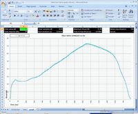
The thrust curve of a rocket motor is a key indicator of its performance. After all it is the generated thrust that propels the rocket skyward. The shape of the curve also gives insight in the inner workings of the motor, and can be used to verify if the design criteria were met. In order to analyse the thrust curve of a static motor test, a thrust curve capture device is used. This device can be thought of as a digital scale, where the weight that is normally shown on the display is instead captured and saved at a fixed interval many times over the duration of the burn.

In fact, the device presented here is in fact just that. It uses a load cell salvaged from a cheap digital scale, of which the weight (and thus the motor thrust exerted upon it) is sampled by the A/D-converter of a microprocessor, and subsequently sent to a laptop computer to be saved into a text file. After the static test is finished, the raw test results can be imported into a spreadsheet for detailed analysis.

The way the system works can best be explained using a block diagram. When the rocket motor is fired, it exerts thrust upon the load cell. This thrust causes the beams of the load cell to flex, thus changing the resistance of the strain gauges attached to it. This change of resistance puts the Wheatstone bridge in a state of non-equilibrium, which causes a small voltage across the bridge. This voltage is amplified by a gain stage, converted from analogue to digital by a micro-controller, and subsequently sent over USB to a laptop computer. The computer stores the captured data in a text file, which is later copied into an Excel sheet by the user for analysis of the data.

Advantages / disadvantages

The test stand as presented has its advantages and disadvantages.

• The salvaged load cell is cheap and easily procurable, and even though it is not the most accurate load cell that one can procure, it is well-suited to its purpose if sufficient care is taken to compensate for its shortcomings.

• Using a micro-controller with built-in A/D-converter and USB interface makes for a very compact and integrated solution. The A/D-converter’s resolution (10 bit) is more than sufficient for this purpose. A load cell of 100 kg will have a resolution of 97 grams.

• The board is supplied with power by the USB interface, which is quite convenient but depending on the quality of the power supply of the computer used, can wreck havoc in the stability of the measurements. Tests have shown that a laptop running on AC power introduced a very noticeable 50Hz ripple onto the sampled data, which however disappears when running on battery power (as would be expected when doing static tests in the field). A separate and well-regulated power supply would be recommended when running the computer on mains power. For this purpose a power-over-USB jumper can be cut on the board. The ripple can also be filtered out in software using a recursive filter.

Schematic

Load cell configuration

Load cells convert force to resistance. They consist of flexible resistors (strain gauges) which are glued to a bending beam type of arrangement. As the beam flexes due to the force that is applied upon it, the strain gauges stretch or compress which causes their resistance to change. Because an A/D-converter cannot read a resistance directly, this change of resistance needs to be converted to a change in voltage by a Wheatstone bridge configuration.

There are several types of load cells, both based upon their physical configuration (bending beam, torsion etc) and on the number of strain gauges employed. The latter can be identified by the number of leads on the load cell.

A full bridge arrangement has 4 strain gauges; two active (which change resistance when force is applied on the load cell), and two passives (which are used solely to balance the bridge). This type of load cell has 4 leads; two for the excitation voltage and two for the signal voltage. The advantage is that this bridge configuration is less prone to output drift caused by temperature changes.

A half-bridge arrangement has only 2 strain gauges, and therefore has three leads; one for the excitation voltage, one for the signal voltage, and a common ground.

Consult Wikipedia for detailed information about the full-bridge Wheatstone and the half-bridge configuration (potential divider).

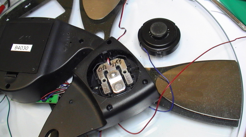
The load cell I used was salvaged from a digital scale, bought on sale for about 15€ in the Aldi supermarkets. When purchasing a scale, it is important to check if the scale actually has 4 load cells. Some scales use an ingeniously designed assembly of levers to transport the load on the 4 edges of the scale to a single load cell in the middle of the scale. Since the load is also scaled down by the levers, these load cells usually have a maximum weight that is too low to be suitable as a static test load cell. My scale had a glass plate with 4 supports on the edges, with only a thin non-transparent cover running from the supports to the display. Since the thin cover couldn’t possibly conceal levers, it was a good bet that each of the 4 supports would hold a load cell. Dividing the max weight of the scale (180kg) by 4 load cells means each load cell was rated at 45kg maximum weight. Perfect for a static test load cell. Similarly, dividing the price by 4 load cells means that each load cell costs 4€.

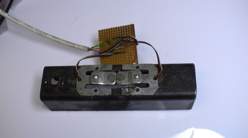
To double the maximum thrust which can be measured, two load cells were mounted side my side on a piece of steel bar. The motor rests on top of this assembly, and the motor’s thrust is transferred to both load cells by a metal plunger which was turned on the lathe. Using two load cells has the advantage of better balancing the Weathstone bridge. Only two passive resistors are necessary. They are mounted on a separate piece of perf board so they can be kept close to the load cells.

As stated above, the bridge arrangement of load cells converts resistance into a voltage. The voltage difference between zero force applied and maximum force applied is quite small however (typically a few tens of a millivolt). It therefore needs to be amplified to a voltage range which is suitable for the A/D-converter. For this a gain stage is used.

Gain section

As a gain stage the AD627 instrumentation amplifier by Analog Devices is used. This choice is largely based on availability. Most load cell amplifier designs on the web seem to use the Burr-Brown INA12x series of instrumentation amplifiers, however I was unable to procure these at a reasonable cost. The AD627 can be sampled for free with a little persuasion, so the price was right.

The amplifier circuit is a pretty straightforward application of the device’s data sheet. Bread boarding the circuit during the design phase showed that two stage amplification was necessary to avoid common mode voltages. I chose to build the circuit with a first stage gain of 200 and a second stage gain that is variable from 1 to 10. It should however be possible to build this circuit with a single gain stage, which I will further investigate.

Since the load cell bridge is not an ideal bridge, it will not be fully balanced even though no force is applied. A small offset voltage will be present, which will be further amplified if not corrected. Therefore it is necessary to zero out the offset voltage. For this a small trimmer pot on the first gain stage’s reference input is used. It can remove most of the offset voltage from the circuit, but since the amplifier is not ideal, a small amount of internal offset voltage will remain. This has proven to be about 2 to 3 ADC bits, which at 0,3% of the useful range is quite acceptable.

A trimmer in the second gain stage allows setting the gain between 1 and 10, resulting in a total gain between 200 and 2000. Depending on the load cell used and its output voltage, the first and/or second gain stage’s gain resistors might have to be changed (by experimentation).

A 100nF and a 1µF capacitor are placed on the power rails of the two instrumentation amplifiers to ensure proper power supply decoupling for these sensitive devices.

Since this amplifier section has a large gain it will readily amplify any noise present to significant levels. Adequate care most be given to reduce these sources of interference. Keeping the cables to the load cell short and keeping the amplifiers away from the micro-processor’s clock signal is necessary.

Micro-controller

The central part of this schematic is a PIC 18F2550 micro-controller by Microchip. It has a built-in 10 bit A/D converter which is used to sample the output of the gain stage and convert it to binary data. In addition it has a built-in USB interface which allows the board to upload data to the computer for capture into a file.

The micro-controller’s schematic is fairly standard for USB implementations. Microchip’s Communication Class Devices (CDC) code is used, so the necessary drivers are included in most recent Windows versions. If you have an unsupported operating system, drivers can be downloaded from Microchip’s website. When connected, the device will show up as a new COM port.

The circuit has a standard ICSP header which can be used to program the micro-controller in the circuit. A reset switch is provided to reset the micro-controller if necessary. There are two LEDs; a power LED and a LED that is used to indicate the status of the program. The second switch is not used in the micro-controllers’ program, and can be omitted.

Buttons and LEDs

The schematic includes a button and two LEDs. The button is not currently used, although it could be used in future firmware revisions for example to start or stop the capture. A button is cheap, both in cost and board real estate, so I always add one.

There is a Reset button on the board as well, which allows the resetting of the micro-controller when necessary. I added this button as it speeds up development, but removing the power has the same effect so for daily use the reset button can be omitted.

The power LED indicates that the board is powered up. The other LED is used to indicate the USB connectivity status. If the board is powered up it will flash rapidly. Once the USB COM port is connected, it will flash twice per second.

Printed Circuit Board

The board is double sided and thus fairly compact. One must not forget to install the two vias, which are located in the amplification section.

The USB connection is provided on a standard .1” pin header, for which a suitable cable must be constructed. I used a USB cable with a type A USB connector, salvaged from an old mouse. It was cut off and soldered to an old floppy drive power connector (which is essentially a 4-pin female header).

A “bus power” jumper has been put on the board. When the jumper is closed the circuit uses the power provided by the USB port from the computer. Power dissipation is less than 100mA. Even though this jumper will probably never be removed, it allows the use of external power if required.

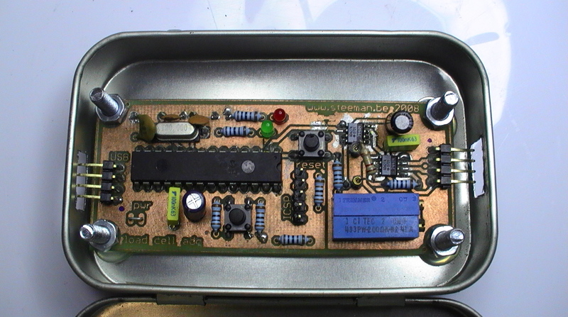
In order to properly shield the circuit from outside interference I have installed it in an Altoids mint tin. A rectangular hole was cut in the side at each end to accommodate the connectors. This case further protects the circuit from burn damage in case of a CATO. The board is mounted on small stand-offs, which were hot-glued into the case. The stand-offs prevent the bottom of the board from shorting out on the tin.

Operating procedure

The operation procedure for the system is as follows.

Connect

Connect the circuit to the USB port of the computer. The power LED should come on solid, and the other LED should flash rapidly, signifying that the serial port is not connected. Connect to the new COM port using a terminal program (e.g.. HyperTerminal). The COM port number will be different for each USB port on the computer, so it is best to always use the same USB port. The terminal settings are 115.200 baud, 8 data bits, no parity, 1 stop bit, no flow control. If the terminal program is connected the LED will flash twice per second, and an intro text will be seen in the terminal program.

Calibrate

The circuit must be calibrated before its first use. Afterwards it might be wise to repeat the calibration regularly if accurate absolute measurements are required.

Null-point reference

First the null-point reference is set. This is done with the motor installed in the test stand. First give a push on the load cell to start the data capture. Numbers will being scrolling on the screen. Now adjust the zero trimmer. As the trimmer is adjusted, the numbers scrolling on the screen will change. Adjust the trimmer until the smallest value is reached. You will notice that any further turning no longer decreases the values. Turn the trimmer back in the other direction to right before the value goes up again. This is the null-point reference sweet spot. It will be filled into the spreadsheet later (‘data’ tab, “ADC base value” cell).

Gain calibration

Next the maximum gain calibration is set. Check the load cell’s maximum rated force (weight), and apply that weight to the load cell, for example by putting barbell weights on it or hanging buckets of water from it. Now adjust the gain trimmer until the values just reach 1023. Note down the weight applied and fill it into the spreadsheet (‘data’ tab, “Load cell max thrust” cell). Mind that the weight as filled into the spreadsheet is expressed in Newton (10kg = 1N).

Make sure no more weight is applied to the load cell than its maximum rating, as this can permanently damage the load cell.

Capture data

To start capturing test data, reset the circuit by disconnecting and re-connecting the USB cable. Re-connect the terminal program and make sure that the start-up text appears.

Set the terminal program to capture to a text file (“Transfer” – “Capture Text” in HyperTerminal). This makes sure that all thrust values captured during the static test are stored into a text file on the computer (e.g. desktop\test 20080221.txt)

After the motor has been fired the text capture function needs to be stopped. Then open the text file and hope that the static test has been captured properly.

Excel sheet

Based on the captured test data, the Excel sheet will be filled out. First the “Input” fields on the “data” tab need to be filled out.

The first line of the captured text file indicates the sample speed of the test (in Hz or samples per second). Fill in this value in the spreadsheet (“data” tab, “Sampling freq” cell). This will always be the same value unless the micro-controller’s firmware is changed. The ADC base value is also shown. This is the null-point reference as set during the calibration. Because this value can vary with temperature and over time it is logged at the start of every static test. Fill in this value from the text file into the spreadsheet (‘data’ tab, “ADC base value” cell).

Fill in the total weight of the propellant in the “Propellant weight” cell. This value is used to calculate the propellant’s ISP after the test.

In the text file, now delete the row of text showing the sample frequency and ADC base value, and select all following text (“ctrl-a”) and copy it to the clipboard (“ctrl-c”). Go to the Excel spreadsheet and find the “Data input area” in the “data” tab. Select the cell directly under the “Data input area” heading, and paste the copied data (“ctrl-v”). This will effectively populate the whole column with the test data. Even though this can be quite a bit of data, it is important to note that the Excel sheet can only process 30.002 rows (due to an Excel limitation).

The spreadsheet now automatically calculates the test data. A thrust graph is shown in the tab “graph”. This graph can be smoothed by applying a built-in filter. To increase the smoothing effect, increase the filter value in the upper left column. This value is effectively the number of samples that are averaged using a recursive filter.

The static test data is shown in the “Outputs” area in the “data” tab. Here you can find information such as the total duration of the burn, total impulse, Isp and avg thrust.

The “Static test identification” field allows the user to enter text to identify the test.

Future improvements

SMD

The next iteration of the board will use all SMD components and will thus be much smaller. The 18F2550 is available in an SOIC package which, with a little persistence and a lot of magnification, shouldn’t be too hard to solder.

Single gain stage

The current version is using a dual gain stage. This is mainly due to my lack of knowledge on how to properly design amplifier circuits. In a future version it must be further investigated how the necessary (configurable) gain can be achieved with just one gain stage, while keeping common mode voltages low.

Input for igniter voltage which can start data capture

Currently the firmware detects the start of the static test by looking for a sudden increase in force on the load cell. This means that it misses around 0,5ms at the start of the test. This is not really an issue for the thrust graph or the total thrust calculations, but it is detrimental to the accuracy of the total burn time, and thus also the calculation of the propellant’s ISP. Additionally, if the motor under test does not come up to pressure immediately after ignition, the capture of the test data will only start when the motor comes up to pressure and starts generating thrust.

It might thus be better to have an input that signals that the ignition has started. In a future version of the load cell amp, a micro-controller input pin will be connected to the voltage that drives the igniter. This way the data capture can start as soon as the power is applied to the igniter, which ensures that the full useful range of data is captured.

Increase sample speed

Even though the sample speed of 6000Hz is plenty for the intended goal, it should be possible to increase this speed to 10.000Hz. Currently the firmware sends the ADC value directly over the USB connection, which means 4 characters for an ADC value of 1023. The transmission of these characters is the limiting factor. When increasing the sample speed, the USB connection would get congested, unless the number of transmitted characters is decreased. This can be done by sending the difference between two samples instead of the whole sample value. The difference between two samples would typically be a 2 digit number or less.

Resources

Schematic & board in Eagle

• DIP version
• SMD version NOT TESTED
• Schematic representation of how the load cells in my digital scale were connected, and the equivalent schematic used for the load cell amplifier

Firmware

• Source code and HEX file (in CCS C)
• USB driver (Microchip CDC driver)

Analysis spreadsheet (Excel)

• Excel spreadsheet

Static test video

Here are some videos that demonstrate the capabilities of the system.

• 20080210 test A
• 20080210 test B

License

Please benefit from my work in your own projects! The firmware for this project is available under a GPL v2 license (as described in the source file), the hardware is available under the TAPR Open Hardware License v1.0.

Comments